Stablepools Are Boring? You're Wrong.

Exploring stablecoin pools on Uniswap v3 - price, volatility, correlation, and more...

Someone told us that stablecoin pools were boring😬🤯 Here's why they're wrong!👇

For starters, around 1B out of 3.7B TVL in Uni v3 is a stablecoin pool. That's around 27%! Of that 1B, about half of it (0.45B) is concentrated in the DAI-USDC pools at 0.01% and 0.05%. But it's not just about size. Let's dig deeper into some of these pools.

We investigate the following UniV3 pools:

• USDC-USDT (0.01%)

• USDC-USDT (0.05%)

• USDC-DAI (0.01%)

• USDC-DAI (0.05%)

• FRAX-USDC (0.05%)

(Psst! See 👇 for a tutorial on obtaining pool data using Python and GBQ 😉)

Panoptic @Panoptic_xyz

Read our latest #ResearchBite from @_DoctorC_ of the @Panoptic_xyz research team! ====== It can be challenging to access data from the Ethereum blockchain. How do we do it? Here's a tutorial about how to fetch data using @Google's BigQuery and their public Ethereum database 👇

Doctor C. @_DoctorC_

1/8 #ResearchBites Have you ever wondered how to obtain historical UNIV3 data? 🧵

Let's start by looking at prices. They should be super stable...right?

Mostly! Some stable pools are more stable than others 🐷🏠

Some pools exhibit short periods of large variability, likely due to whales + MEV + UniV3 liquidity math (e.g. USDC-USDT 0.05%)

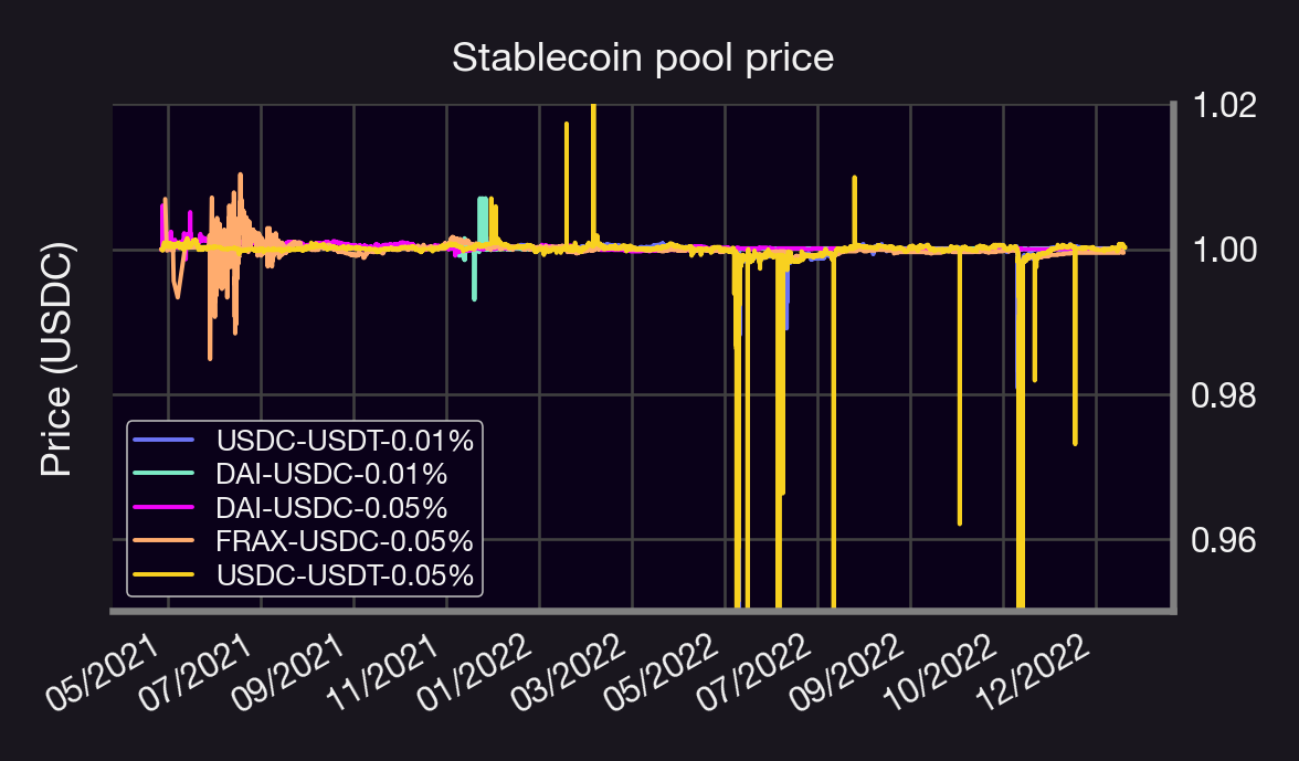
Remark: The prices 👆 are ordered on a "per-tx" basis; thus, some of the larger spikes happen inside the same block as their neighboring transactions.

Some pool stats:

• Most stable: DAI-USDC (0.01%)

• Most popular: USDC-USDT (0.01%)

• Largest volatility: USDC-USDT (0.05%)

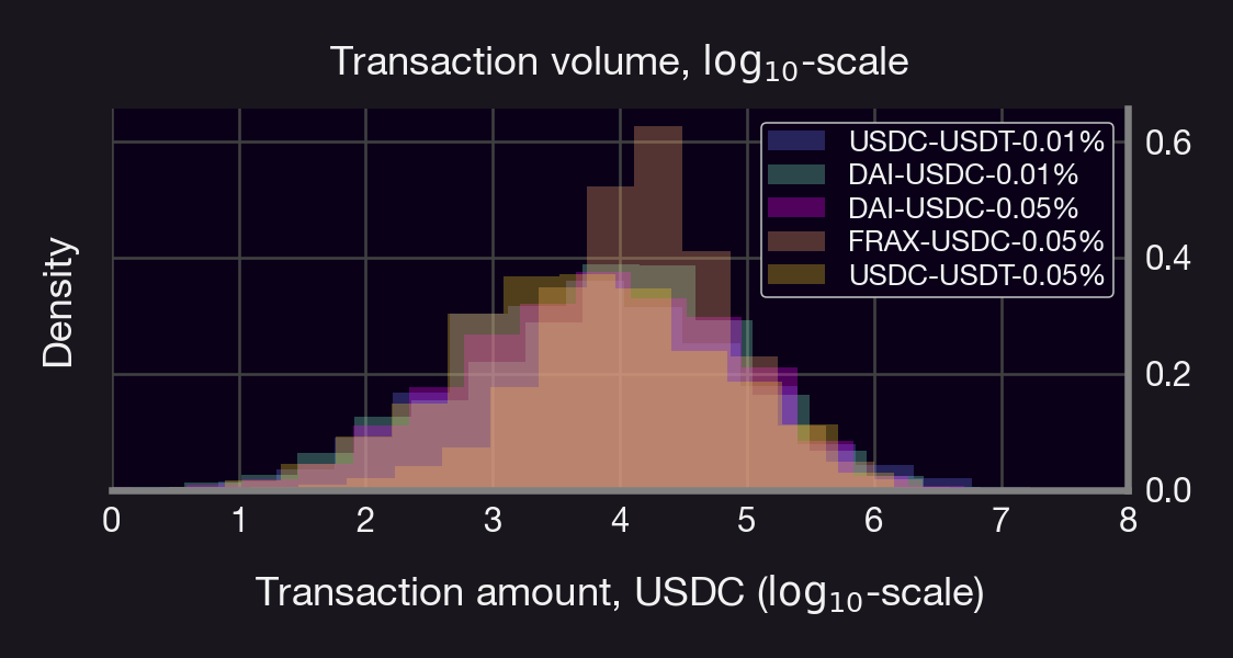
• ~Log-normal distribution of txs (eyeballing it)

• See histograms + summary statistics👇

(Note: here ~ means "approximately")

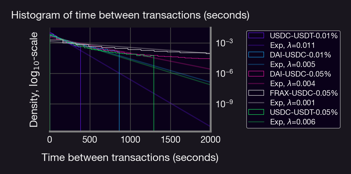
What about time between txs?

• USDC-USDT (0.01%) is the busiest pool (~1 tx/min on avg)

• FRAX-USDC (0.05%) is the quietest pool

• Each distribution resembles a geometric (and hence exponential) distribution with a given parameter λ (but with fatter tails)

See figs👇

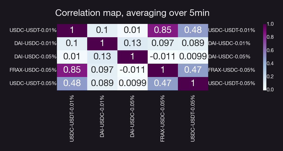
Now let's examine price correlation b/t pools:

• Since txs occur at irregular intervals, we take the avg price over 5 minute intervals

• Not all are as strongly correlated as one would think 🤔

• High correlation b/t USDC-{USDT,FRAX} pools

• Low correlation for DAI pairs

Key insights:

• Per tx price is less stable than one would think!

• There is, on average, ~1 tx every 5 minutes across all pools

• Tx amount ~log-normal; time between txs ~exponential

• Price across some pools are weakly correlated, with Dai being the odd one out

Why is this important?

• Understanding the behavior of stablecoin pools can help us model them (e.g. for forward testing); can't use GBM

• Understanding correlations b/t pools can help us develop beta-trading strategies (e.g. stat-arb) (👆topics of future #ResearchBites)

Why can't we use GBM? Intuitively, stablecoins should:

• Oscillate around 1 (e.g., USDC)

• Have bounded variation (not stable otherwise)

Whereas for GBM:

• Price either becomes unbounded (µ>0) or goes to 0 (µ<0) in expectation

• Variance increases with time 👇🤓

Indeed, let S denote an asset with price process {S}. Furthermore, let μ denote the drift parameter of the price process and σ>0 its volatility, and let W denote the standard Wienner process. We say that {S} follows a Geometric Brownian motion (GBM) if {S} satisfies the following stochastic differential equation:

\(\begin{align}\\ \frac{\mathrm{d}S_t}{S_t}&=\underbrace{\mu\mathrm{d}t}_\text{drift}+\underbrace{\sigma\mathrm{d}W_t}_\text{volatility},\\ \text{with }& W_t \text{ Gaussian noise} \end{align}\)

Furthermore, given an initial price S0, it follows from Ito’s lemma that

\(S_t=S_0\exp\left(\left(\mu-\frac{\sigma^2}{2}\right)t+\sigma W_t\right), \quad \forall t\geq 0\)

Which in turn implies that its mean and variance are given by:

\(\begin{align} \mathbb{E}[S_t]&=S_0e^{\mu t}\\ \mathbb{V}[S_t]&=S^2_0e^{2\mu t}(e^{\sigma^2t}-1)\\ \end{align}\)

which, as we can see, increase as t increases! This is clearly not the case for stable coins.

Disclaimer: This content is for educational purposes only and should not be relied upon as financial advice. Please DYOR!